※ Elliott Pattern Helper Add In
- Download Add In for Excel 2007 ☞
- Download Add In for Excel 2003 ☞
▶ Multiresolution Analysis with Wavelet Transform
파동은 상이한 진폭과 상이한 주기(또는 주파수)를 갖는 다수의 신호들이 복합된 것(composite signal)이라고 볼 수 있다. 예를 들어 다음의 파동을 관찰해 보자.
 |
| 그림 1. Composite signal |
많은 노력을 들이지 않더라도 그림 1의 파동은 다음 그림 2의 파동 (a), (b)와 (c)를 합쳐 놓은 것이라는 것을 알 수가 있다.
 |
| 그림 2 |
Multiresolution analysis 또는 Multiscale approximation은 위의 관점에서 파동을 해체한 후, 파동을 특정 resolution(또는 scale)의 approximation과 그 보다 낮은 resolution의 detail coefficient들로 재구성한다. ※ 자세한 사항은 Wavelet Transform 관련 서적을 참고하십시요.
▶ Multiresolution Decomposition
다음 그림은 특정 시계열 데이터에 대해 multiresolution decomposition을 수행한 결과를 보여 준다. (Haar a trous transform, scale 5)
 |
| 그림 3-1. Approximation at scale 5 |
 |
| 그림 3-2. Detail coefficients at scale 1 |
 |
| 그림 3-3. Detail coefficients at scale 2 |
 |
| 그림 3-4. Detail coefficients at scale 3 |
 |
| 그림 3-5. Detail coefficients at scale 4 |
 |
| 그림 3-6. Detail coefficients at scale 5 |
위 그림 3의 6개 파동을 모두 합치면 어떤 모양이 될까? 위 decomposition 결과를 가지고 역으로 원래의 파동을 reconstruction하면 다음 그림 4의 결과를 얻을 수 있다.
 |
| 그림 4. Reconstruction |
어디서 많이 본 듯한 파동의 모양이 아닌가? 그렇다. 바로 KOSPI 지수의 최근 140 거래일 동안의 파동이다. ※ 주의: 종가 기준이 아니라 고가와 저가의 평균가 기준임
▶ Dimensionality Reduction
우리가 주식 시장에서 접하는 파동들은 분 단위, 시간 단위, 일 단위, 주 단위, 월 단위 등 time scale에 상관 없이 그림 4와 유사한 모양을 갖는다.
Glenn Neely의 파동 분석 방법은 '중요한 저점 또는 고점'에서 시작된 일련의 monowave들의 구조 및 진행기호 분석에서 시작된다. Elliott Pattern Helper(EPH)를 이용하여 위 chart에서 monowave들을 추출하면 다음 그림과 같다.
 |
| 그림 5. Monowaves |
가령 그림 5와 같이 박스 A로부터 monowave 분석을 시작해 나갈 수도 있을 것이며, 그림 6과 같은 중간 결과를 얻을 수도 있을 것이다.
 |
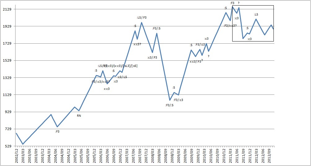
| 그림 6. Structure/progress notation of monowaves |
그런데, 파동 분석이 어려운 이유 중의 하나는, 그림 6에서 간파했을지도 모르겠지만, 하나의 파동에 다양한 degree의 패턴이 뒤죽박죽 섞여 있다는 것이다.
그림 6의 파동 중간에 위치한 작은 monowave 7개를 관찰해 보자. 각각은 그 이전 monowave와 비교했을 때 시간 및 길이에서 확연한 차이가 난다. 즉, 쉽게 생각해서 degree가 다르다고 볼 수 있는데, 이들의 구조 및 진행기호를 하나씩 하나씩 분석해 나가야 할까?
이렇듯 우리는 파동 분석 과정에서 'dimensionality curse'를 겪을 수밖에 없는데, 이를 회피할 방법은 없을까?
이번 글의 제목이자 주제인 바, dimensionality reduction이 이 문제의 해결을 위한 수단이 되지 않을까 생각해 본다.
어떻게 보면, 큰 추세와는 상관이 없어 보이는 작은 파동들을 하나로 묶어 의미있는 파동 패턴을 쉽게 찾을 수 있도록 하는 방법이라고 볼 수도 있겠다.
▶ Transform and Filtering
위에서 언급한 Haar a trous wavelet transform과 filtering을 적용한 후 EPH를 통해 구조/진행기호를 분석한 결과는 다음과 같다.
 |
| 그림 7-1. Before wavelet transform |
 |
| 그림 7-2. After wavelet transform, layer 1 filtering |
 |
| 그림 7-3. After wavelet transform, layer 1 & 2 filtering |
그림 7-1에서 7-3까지, 'curse'로부터 벗어나기 위한 노력이 가치가 있을까? Daily chart가 아닌 weekly chart, weekly chart보다 더 긴 시간 단위의 monthly chart를 볼 때와는 달리 detail을 포기하지 않아도 될 듯한데...
※ 그림 1과 2는 'The Illustrated Wavelet Transform Handbook, Paul S. Addison'에서 차용한 것임을 밝힙니다.